class: center, middle, inverse, title-slide .title[ # <b>Statistical Analysis Strategies for Eye-Tracking Data</b> ] .subtitle[ ## Eye tracking technology: A training workshop on methods for psychological and educational research<br><br> ] .author[ ### Dan Mirman<br>dan[at]danmirman.org ] .institute[ ### Department of Psychology<br>The University of Edinburgh ] .date[ ### 10 May 2022 ] --- # Overview Eye-tracking provides very rich data with high temporal resolution. This richness is great for us as cognitive psychologists, but it presents a challenge for analysis. This talk: some of those challenges, different strategies for tackling them, and the strengths and weaknesses of those different strategies. 1. (G)LMEM: (Generalised) Linear Mixed Effects Modeling 2. GCA: Growth Curve Analysis 3. GAMM: Generalised Additive Mixed Models 4. Cluster-Based Permutation in Time (cbpt) --- # Eye-tracking measures from reading tasks This morning, you learned from Victor Kuperman about using eye-tracking to study reading. Some typical measures: * Gaze durations: First fixation duration, First gaze duration, Total fixation time + continuous, positive * Regressions (into word, out of word), refixations on first pass, skips + binary -- ### From a statistical analysis perspective These are like other outcome measures (RT, accuracy), but * more dense (multiple outcomes per trial) * nested: multiple observations per participant (across items) and items (across participants) --- # (G)LM: (Generalised) Linear Modeling .pull-left[ <!-- --> ] -- .pull-right[ `\(Y_{ij} = \beta_{0} + \beta_{1} \cdot X_{j} + \epsilon_{ij}\)` __Fixed effects__: <span style="color:blue"> `\(\beta_{0}\)` </span> (Intercept), <span style="color:red"> `\(\beta_{1}\)` </span> (Slope) __Residual error__: `\(\epsilon_{ij}\)` ] --- ## (G)LMEM: (Generalised) Linear Mixed Effects Modeling .pull-left[ <!-- --> __Nested observations__: Observations that come from the same participant (or item) are likely to have a shared pattern * A fast participant will have consistently short RT across items * A difficult item will have consistently longer RT and/or more errors (longer fixations, fewer skips, etc.) ] .pull-right[ `\(Y_{ij} = \beta_{0i} + \beta_{1} \cdot X_{j} + \epsilon_{ij}\)` __Fixed effects__: <span style="color:blue"> `\(\beta_{0}\)` </span> (Intercept), <span style="color:red"> `\(\beta_{1}\)` </span> (Slope) __Residual error__: `\(\epsilon_{ij}\)` ] --- ## (G)LMEM: (Generalised) Linear Mixed Effects Modeling .pull-left[ <!-- --> __Nested observations__: Observations that come from the same participant (or item) are likely to have a shared pattern * A fast participant will have consistently short RT across items * A difficult item will have consistently longer RT and/or more errors (longer fixations, fewer skips, etc.) ] .pull-right[ `\(Y_{ij} = \beta_{0i} + \beta_{1} \cdot X_{j} + \epsilon_{ij}\)` __Fixed effects__: <span style="color:blue"> `\(\beta_{0}\)` </span> (Intercept), <span style="color:red"> `\(\beta_{1}\)` </span> (Slope) __Residual error__: `\(\epsilon_{ij}\)` `\(Y_{ij} = \beta_{0i} + \beta_{1} \cdot X_{j} + \zeta_{0i} + \zeta_{1i} + \epsilon_{ij}\)` __Random effects__ * `\(\zeta_{0i}\)` participant-specific variance in *intercept* * `\(\zeta_{1i}\)` participant-specific variance in *slope* * Random effects require a lot of data to estimate We assume these are randomly sampled from a population of participants (and items), so they should have a normal distribution around the overall group means ( `\(\beta_{0}\)` and `\(\beta_{1}\)` ). ] --- # Fixed vs. Random effects ### Fixed effects * Interesting in themselves * Reproducible fixed properties of the world (nouns vs. verbs, WM load, age, etc.) * <span style="color:red"> *Unique, unconstrained parameter estimate for each condition* </span> -- ### Random effects * Randomly sampled observational units over which you intend to generalize (particular nouns/verbs, particular individuals, etc.) * Unexplained variance * <span style="color:red"> *Drawn from normal distribution with mean 0* </span> --- # Example: Reading compound words <!-- --> --- # Example: Reading compound words ```r library(lme4) library(lmerTest) mod_complex <- lmer(GD ~ CompoundLength + (1 + CompoundLength || SubjectID) + (1 | Compound), data=dat_complex) ``` -- ```r coef(summary(mod_complex)) ``` ``` ## Estimate Std. Error df t value Pr(>|t|) ## (Intercept) 202.89 12.565 953 16.15 5.010e-52 ## CompoundLength 16.97 1.479 1024 11.47 9.651e-29 ``` -- ```r VarCorr(mod_complex) ``` ``` ## Groups Name Std.Dev. ## Compound (Intercept) 47.74 ## SubjectID CompoundLength 8.71 ## SubjectID.1 (Intercept) 55.68 ## Residual 153.79 ``` --- # Resources There are tons of books, papers, online tutorials, etc. about mixed effects modeling (aka multilevel modeling, hierarchical linear modeling). A few that I have found particularly useful: * Alexander Demos: course notes from Applied Mixed-Effects Models http://www.alexanderdemos.org/MixedOverview.html * Violet A. Brown (2021). An introduction to linear mixed-effects modeling in R. _Advances in Methods and Practices in Psychological Science, 4_(1), 2515245920960351. https://doi.org/10.1177/2515245920960351 * Meteyard, L., & Davies, R. A. (2020). Best practice guidance for linear mixed-effects models in psychological science. _Journal of Memory and Language, 112_, 104092. https://doi.org/10.1016/j.jml.2020.104092 * Brauer, M., & Curtin, J. J. (2018). Linear mixed-effects models and the analysis of nonindependent data: A unified framework to analyze categorical and continuous independent variables that vary within-subjects and/or within-items. _Psychological Methods, 23_(3), 389-411. https://doi.org/10.1037/met0000159 * Luke, S. G. (2017). Evaluating significance in linear mixed-effects models in R. _Behavior Research Methods, 49_(4), 1494-1502. https://doi.org/10.3758/s13428-016-0809-y --- # Non-linear effects (G)LMEM are great when the effects are (approximately) linear What about non-linear effects? -- A common case: non-linear time course of fixation  The "Visual World Paradigm", or fixations during spoken word-to-picture matching --- # GCA: Growth Curve Analysis An extension of (G)LMEM, widely used in longitudinal data analysis -- Key enhancement: polynomial transformation of predictors to capture non-linear relationships *Caveat: Polynomials are good mathematically, but not great cognitively and not good for capturing complex curve shapes (more on this later)* -- **Example 1: Time course of fixations** <!-- --> --- # Example 1: Time course of fixations ```r mod_semcomp <- lmer(FixProp ~ (poly1+poly2+poly3+poly4)*Condition + (poly1+poly2+poly3+poly4 | Subject) + (poly1+poly2+poly3+poly4 | Subject:Condition), data=subset(dat_semcomp, Object == "Competitor"), REML=FALSE) ``` -- .scroll-output[ |effect |term | estimate| std.error| statistic| df| p.value| |:------|:----------------------|--------:|---------:|---------:|------:|-------:| |fixed |(Intercept) | 0.1123| 0.0084| 13.3209| 112.61| 0.0000| |fixed |poly1 | -0.2698| 0.0298| -9.0672| 108.35| 0.0000| |fixed |poly2 | 0.0167| 0.0257| 0.6514| 111.53| 0.5161| |fixed |poly3 | 0.0450| 0.0198| 2.2733| 113.54| 0.0249| |fixed |poly4 | -0.0176| 0.0197| -0.8942| 104.80| 0.3733| |fixed |ConditionDistant | 0.0360| 0.0114| 3.1457| 80.32| 0.0023| |fixed |ConditionNear | 0.0700| 0.0114| 6.1207| 80.32| 0.0000| |fixed |poly1:ConditionDistant | 0.0164| 0.0385| 0.4245| 77.76| 0.6724| |fixed |poly1:ConditionNear | 0.1245| 0.0385| 3.2301| 77.76| 0.0018| |fixed |poly2:ConditionDistant | 0.0194| 0.0344| 0.5645| 95.47| 0.5737| |fixed |poly2:ConditionNear | -0.1110| 0.0344| -3.2286| 95.47| 0.0017| |fixed |poly3:ConditionDistant | -0.0286| 0.0274| -1.0446| 94.77| 0.2989| |fixed |poly3:ConditionNear | -0.0410| 0.0274| -1.5003| 94.77| 0.1369| |fixed |poly4:ConditionDistant | 0.0157| 0.0247| 0.6355| 76.01| 0.5270| |fixed |poly4:ConditionNear | 0.0662| 0.0247| 2.6776| 76.01| 0.0091| ] --- # Example 2: Time course of pupil dilation <!-- --> --- # Example 2: Time course of pupil dilation ```r mod_pupil <- lmer(baselinep ~ (poly1+poly2+poly3)*txthm*hilo + ((poly1+poly2+poly3)+txthm*hilo|subject), contrasts = list(txthm="contr.sum", hilo="contr.sum"), data=dat_pupil, REML=FALSE) ``` .scroll-output[ |effect |term | estimate| std.error| statistic| df| p.value| |:------|:------------------|--------:|---------:|---------:|-------:|-------:| |fixed |(Intercept) | 0.0644| 0.0117| 5.5058| 59.52| 0.0000| |fixed |poly1 | 0.1154| 0.0350| 3.2977| 59.67| 0.0016| |fixed |poly2 | -0.0655| 0.0209| -3.1299| 52.79| 0.0028| |fixed |poly3 | 0.0089| 0.0164| 0.5426| 56.37| 0.5896| |fixed |txthm1 | 0.0007| 0.0043| 0.1665| 61.04| 0.8683| |fixed |hilo1 | -0.0022| 0.0041| -0.5250| 61.10| 0.6015| |fixed |poly1:txthm1 | 0.0134| 0.0067| 1.9904| 4316.09| 0.0466| |fixed |poly2:txthm1 | 0.0084| 0.0065| 1.2890| 4292.31| 0.1975| |fixed |poly3:txthm1 | -0.0064| 0.0063| -1.0087| 4257.49| 0.3132| |fixed |poly1:hilo1 | -0.0193| 0.0067| -2.8669| 4318.81| 0.0042| |fixed |poly2:hilo1 | -0.0141| 0.0065| -2.1529| 4298.37| 0.0314| |fixed |poly3:hilo1 | 0.0043| 0.0063| 0.6749| 4262.85| 0.4998| |fixed |txthm1:hilo1 | -0.0017| 0.0044| -0.3793| 60.59| 0.7058| |fixed |poly1:txthm1:hilo1 | -0.0183| 0.0067| -2.7361| 4313.34| 0.0062| |fixed |poly2:txthm1:hilo1 | -0.0178| 0.0065| -2.7357| 4285.73| 0.0062| |fixed |poly3:txthm1:hilo1 | -0.0033| 0.0063| -0.5282| 4250.33| 0.5974| ] --- # Resources .pull-left[ GCA book <img src="./GCA_book.jpg" height="400px" /> ] -- .pull-right[ ### Tutorials * GCA: https://dmirman.github.io/GCA/index.html * Eye-tracking data analysis (includes data wrangling and pre-processing): https://dmirman.github.io/ET2019.html ] --- # GCA Bottom Line 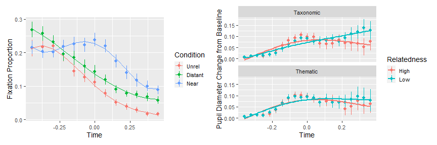<!-- --> GCA works well when trying to fit fairly simple curve shapes and interested in overall trajectories. -- Does not work so well with: 1. Complex curve shapes 2. Identifying time windows where curves are different --- # GAMMs: Generalised Additive Mixed Models * Similar to GCA: mixed effects models, non-linear time course components * Different from GCA: use splines (instead of polynomials), which are much more flexible but trickier in some ways -- **Example**: Timing of function vs thematic semantic competition 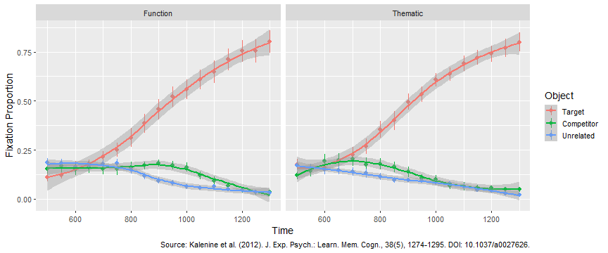<!-- --> --- # Example: Timing of function vs thematic semantic competition ```r # load libraries library(mgcv) # gamm library(itsadug) # for estimating diffs # fit model of Function competition m_funct <- bam(meanFix ~ Object + s(Time) + s(Time, by=Object, k=8) + s(Time, Subject, bs="fs", m=1, k=8), data=subset(FunctTheme, Object!="Target" & Condition=="Function")) # fit model of Thematic competition m_theme <- bam(meanFix ~ Object + s(Time) + s(Time, by=Object, k=8) + s(Time, Subject, bs="fs", m=1, k=8), data=subset(FunctTheme, Object!="Target" & Condition=="Thematic")) ``` **Note that it is not possible to model an Object by Relation Type interaction** --- # Example: Timing of function vs thematic semantic competition .pull-left[ **Function** 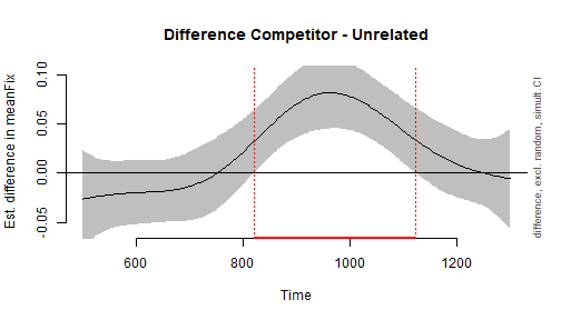<!-- --> Time window of significant difference: 821.6 - 1123.1 ] .pull-right[ **Thematic** 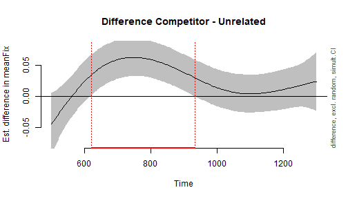<!-- --> Time window of significant difference: 616.6 - 934.2 ] --- # Resources * Wood, S. N. (2006). Generalized Additive Models: An Introduction with R. Chapman and Hall/CRC. https://doi.org/10.1201/9781315370279 * Winter, B., & Wieling, M. (2016). How to analyze linguistic change using mixed models, Growth Curve Analysis and Generalized Additive Modeling. Journal of Language Evolution, 1(1), 7-18. https://doi.org/10.1093/jole/lzv003 * Soskuthy, M. (2017). Generalised additive mixed models for dynamic analysis in linguistics: A practical introduction. arXiv preprint arXiv:1703.05339. https://arxiv.org/pdf/1703.05339.pdf *Problem: can't do interactions* --- # Cluster-based permutation in time Core idea: conduct bin-by-bin statistical tests and detect clusters of time points where effect is significant. Use data permutation to derive a null distribution of cluster sizes. This approach is widely used in neuroimaging to define minimum *spatial* cluster size, i.e., number of voxels; the logic is the same, except defining clusters in time. Very flexible - can be used with any statistical test (e.g., (G)LMEM) at the bin level and produces specific time windows (clusters) where effect is significant. -- ### General strategy 1. Conduct 2x2 rmANOVA in each time bin, detect clusters and calculate cluster mass statistic (CMS). 2. For a large number of runs: + Permute data (while respecting exchangeability under null hypothesis) + Re-conduct analysis and store maximum CMS 3. Calculate p-values by comparing original (observed) CMS to null distribution of maximum CMS --- # Example: Timing of function vs thematic semantic competition .pull-left[ ```r # load libraries library(exchangr) library(clusterperm) # original model m_bin <- aov_by_bin(subset(FunctTheme, Object!="Target"), Time, meanFix ~ Condition*Object + Error(Subject)) orig <- detect_clusters_by_effect(m_bin, effect, Time, stat, p) # cluster-based permutation for Object effects dat_obj <- nest(subset(FunctTheme, Object!="Target"), -Subject, -Object) nhds_obj <- cluster_nhds(1000, dat_obj, Time, meanFix ~ Condition*Object + Error(Subject), shuffle_each, Object, Subject) # get p-values pvalues(orig, nhds_obj) ``` ] -- .pull-right[ |effect | b0| b1| sign| cms| p| |:----------------|---:|----:|----:|------:|------:| |Condition | NA| NA| NA| 0.000| 1.0000| |Object | 500| 500| -1| 4.555| 0.4695| |Object | 850| 1000| 1| 49.381| 0.0020| |Condition:Object | 700| 700| -1| 4.409| 0.4356| |Condition:Object | 950| 1050| 1| 15.879| 0.1449| ] --- # Resources * Barr, D. (2019) https://talklab.psy.gla.ac.uk/barr_eslp_attlis/ + R packages: + `clustperm` (https://github.com/dalejbarr/clusterperm) + `exchangr` (https://github.com/dalejbarr/exchangr) * Yu, C. L., Chen, H. C., Yang, Z. Y., & Chou, T. L. (2020). Multi-time-point analysis: A time course analysis with functional near-infrared spectroscopy. Behavior Research Methods, 52(4), 1700-1713. https://doi.org/10.3758/s13428-019-01344-9 --- # Recap Four statistical analysis strategies for analysing eye-tracking data |Approach |Categorical or Linear Effects Only |Non-Linear Effects |Interactions |Trajectories |Complex Curve Shapes |Identify Signif Time Windows | |:--------|:----------------------------------|:------------------|:------------|:------------|:--------------------|:----------------------------| |(G)LMEM |✅ |❌ |✅ |❌ |❌ |❌ | |GCA |✅ |✅ |✅ |✅ |❌ |❌ | |GAMM |✅ |✅ |❌ |✅ |✅ |✅ | |CBPT |✅ |✅ |✅ |❌ |✅ |✅ | -- ### Thank you .pull-left[ Contact: dan@danmirman.org http://www.danmirman.org | http://dmirman.github.io/ ] .pull-right[  ]